Definition of Aggregate Demand: Aggregate demand (AD) = total spending on goods and services
List of components of aggregate demand: AD = C + I + G + (X-M)
C: Consumers' expenditure on goods and services: Also known as consumption, this includes demand for durables e.g. audio-visual equipment and vehicles & non-durable goods such as food and drinks which are “consumed” and must be re-purchased.
I: Capital Investment – This is spending on capital goods such as plant and equipment and new buildings to produce more consumer goods in the future. Investment includes spending on working capital such as stocks of finished and semi-finished goods.
A small part of investment spending is the change in the value of stocks. Producers may find either than demand is running higher than output (i.e. stocks will fall) or that demand is weaker than expected and below current output (in which case the value of stocks will rise.)
G: Government Spending – This is spending on state-provided goods and services including public goods and merit goods. Decisions on how much the government will spend each year are affected by developments in the economy and the political priorities of the government.
Transfer payments in the form of benefits are not included in current government spending because they are a transfer from one group (i.e. people paying income taxes) to another (i.e. pensioners drawing their state pension having retired, or families on low incomes).
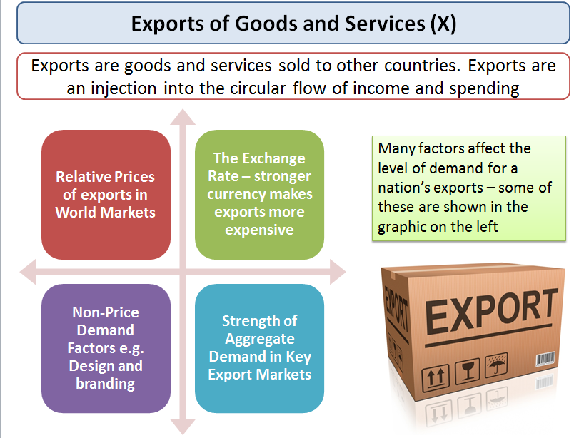
X: Exports of goods and services - Exports sold overseas are an inflow of demand (an injection) into our circular flow of income and spending adding to aggregate demand.
M: Imports of goods and services. Imports are a withdrawal of demand (a leakage) from the circular flow of income and spending.
Net exports measure the value of exports minus the value of imports. When net exports are positive, there is a trade surplus (adding to AD); when net exports are negative, there is a trade deficit (reducing AD).
How changes in the components shift the curve:
Changes in Expectations Current spending is affected by anticipated income and inflation
Changes in Monetary Policy – i.e. a change in interest rates
Changes in Fiscal Policy Fiscal Policy refers to changes in government spending, taxation and borrowing
Economic events in the world economy International factors such as the exchange rate and foreign income
Changes in household wealth
Changes in the supply of credit
Picture of an aggregate Demand Curve:
List of components of aggregate demand: AD = C + I + G + (X-M)
C: Consumers' expenditure on goods and services: Also known as consumption, this includes demand for durables e.g. audio-visual equipment and vehicles & non-durable goods such as food and drinks which are “consumed” and must be re-purchased.
I: Capital Investment – This is spending on capital goods such as plant and equipment and new buildings to produce more consumer goods in the future. Investment includes spending on working capital such as stocks of finished and semi-finished goods.
A small part of investment spending is the change in the value of stocks. Producers may find either than demand is running higher than output (i.e. stocks will fall) or that demand is weaker than expected and below current output (in which case the value of stocks will rise.)
G: Government Spending – This is spending on state-provided goods and services including public goods and merit goods. Decisions on how much the government will spend each year are affected by developments in the economy and the political priorities of the government.
Transfer payments in the form of benefits are not included in current government spending because they are a transfer from one group (i.e. people paying income taxes) to another (i.e. pensioners drawing their state pension having retired, or families on low incomes).
X: Exports of goods and services - Exports sold overseas are an inflow of demand (an injection) into our circular flow of income and spending adding to aggregate demand.
M: Imports of goods and services. Imports are a withdrawal of demand (a leakage) from the circular flow of income and spending.
Net exports measure the value of exports minus the value of imports. When net exports are positive, there is a trade surplus (adding to AD); when net exports are negative, there is a trade deficit (reducing AD).
How changes in the components shift the curve:
Changes in Expectations Current spending is affected by anticipated income and inflation
- When confidence falls, we see an increase in saving and businesses postpone investment projects because of worries over weak demand and lower expected profits.
Changes in Monetary Policy – i.e. a change in interest rates
- If interest rates fall – this lowers the cost of borrowing and the incentive to save, encouraging consumption & investment
- There are time lags between changes in interest rates and AD
Changes in Fiscal Policy Fiscal Policy refers to changes in government spending, taxation and borrowing
- Income tax affects disposable income e.g. lower income tax raises disposable income and should boost consumption.
- A budget deficit is a net injection of aggregate demand
Economic events in the world economy International factors such as the exchange rate and foreign income
- A depreciation in a currency makes imports dearer and exports cheaper - the net result should be that UK AD rises
- An increase in overseas incomes raises demand for exports. In contrast a recession in a major export market will lead to a fall in exports and an inward shift of aggregate demand.
Changes in household wealth
- Changing share and property prices affect the level of wealth
- Declining asset prices can hit confidence / a fall in expectations
Changes in the supply of credit
- The availability of credit is vital for the smooth functioning of most modern economies
- Many banks and other lenders are now more reluctant to lend
- Interest rates on different loans have become more expensive
Picture of an aggregate Demand Curve:
Definition of Aggregate Supply:
is defined as the total amount of goods and services (real output) produced and supplied by an economy’s firms over a period of time. It includes the supply of a number of types of goods and services including private consumer goods, capital goods, public and merit goods and goods for overseas markets.
Components of Aggregate Supply:
Consumer goodsPrivate consumer goods and services, such as motor vehicles, computers, clothes and entertainment, are supplied by theprivate sector, and consumed by households. For a developed economy, this is the single largest component of aggregate supply.
Capital goodsCapital goods, such as machinery, equipment, and plant, are supplied to other firms. These investment goods are significant in that their use adds to capacity, and increases the economy’s ability to supply private consumer goods in the future.
Public and merit goodsGoods and services produced by private firms for use by central or local government, such as education and healthcare, are also a significant component of aggregate supply. Many private firms such as those in construction, IT and pharmaceuticals, rely on contracts to supply to the public sector.
Traded goodsGoods and services for export, such as chemicals, entertainment, and financial services are also a key component of aggregate supply.
How they shift the AS curve.
Different theories of the shape of the AS curve arise from different explanations about how real output responds to changes in aggregate demand. There are, essentially, three different views:
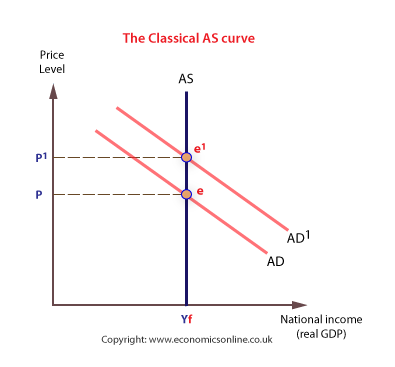
The Classical view of real output was that it was fixed at a particular level. At this level, all the factors of production in the economy would be fully employed.(Say at output 500.)
Changes in AD will only bring about changes in the price level, not the level of real output.
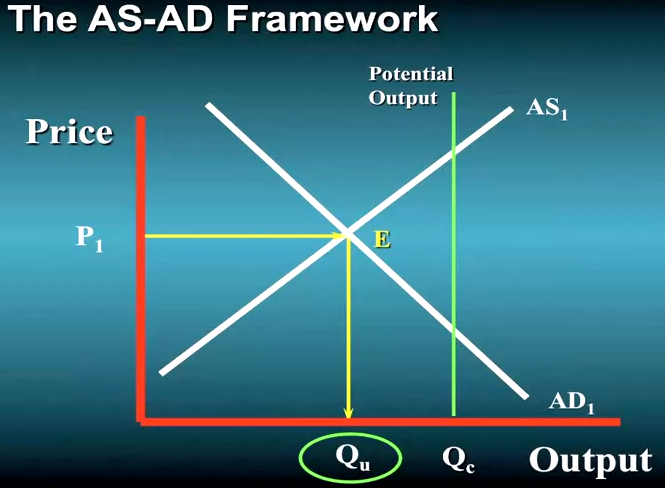
The Keynesian viewThe Keynesian AS curve assumes that prices and wages are fixed until full employment is reached. Over the ‘Keynesian range’ there is spare capacity in the economy, the price level is stable, and real output can expand as a result of increases in AD without any inflationary pressure.
Beyond full employment, any changes in AD will bring about higher price levels. The Keynesian view of AS was adapted to show an ‘intermediate range’ where both unemployment and inflation could occur together.
The adapted Keynesian AS curve is more realistic, and highlights the trade-offs that can occur between the price level and unemployment.
The ‘modern’ short run-long run viewTo solve the problem of the Keynesian and Classical AS curve, modern economists tend to separate the short run AS curve (SRAS) from the long run AS (LRAS) curve. The short run is assumed to begin immediately after an increase in the price level (for example, as a result of an increase in AD), and ends when input prices (costs of production) have increased. Hence, during the short run producers are experiencing an increase in their ‘real’ prices and produce more output – and the supply curve slopes upwards.
Any increase in input prices (costs) which may follow is assumed to lag behind increases in the general price level. In this analysis, SRAS and LRAS are separated. This allows economists to be more flexible in their analysis of a modern economy.
Shifts in the SRASThe most likely cause of a shift in the SRAS curve is to accommodate changes in the short run AD curve.
Shifts in the LRASThe long run aggregate supply curve (LRAS) is the long run level of real output which is sustainable given the current quantity and quality of the economy's scarce resources. Real output in the long run is not determined by the price level, and the long run AS curve will be vertical - short run changes in the price level do not alter an economy’s long-term output. This is equivalent to being on the edge of a country’s production possibility frontier.
The long run aggregate supply curve (LRAS) is shown as a vertical curve, at full employment. LRAS can shift if the economy’s productivity changes, either through an increase in the quantity of scarce resources, such as inward migration or organic population growth, or improvements in the quality of resources, such as through better education and training.
Shifts in LRAS are usually gradual and anticipated, unlike shifts in the SRAS which can be dramatic and unanticipated. LRAS can shift for many reasons, including:
is defined as the total amount of goods and services (real output) produced and supplied by an economy’s firms over a period of time. It includes the supply of a number of types of goods and services including private consumer goods, capital goods, public and merit goods and goods for overseas markets.
Components of Aggregate Supply:
Consumer goodsPrivate consumer goods and services, such as motor vehicles, computers, clothes and entertainment, are supplied by theprivate sector, and consumed by households. For a developed economy, this is the single largest component of aggregate supply.
Capital goodsCapital goods, such as machinery, equipment, and plant, are supplied to other firms. These investment goods are significant in that their use adds to capacity, and increases the economy’s ability to supply private consumer goods in the future.
Public and merit goodsGoods and services produced by private firms for use by central or local government, such as education and healthcare, are also a significant component of aggregate supply. Many private firms such as those in construction, IT and pharmaceuticals, rely on contracts to supply to the public sector.
Traded goodsGoods and services for export, such as chemicals, entertainment, and financial services are also a key component of aggregate supply.
How they shift the AS curve.
Different theories of the shape of the AS curve arise from different explanations about how real output responds to changes in aggregate demand. There are, essentially, three different views:
The Classical view of real output was that it was fixed at a particular level. At this level, all the factors of production in the economy would be fully employed.(Say at output 500.)
Changes in AD will only bring about changes in the price level, not the level of real output.
The Keynesian viewThe Keynesian AS curve assumes that prices and wages are fixed until full employment is reached. Over the ‘Keynesian range’ there is spare capacity in the economy, the price level is stable, and real output can expand as a result of increases in AD without any inflationary pressure.
Beyond full employment, any changes in AD will bring about higher price levels. The Keynesian view of AS was adapted to show an ‘intermediate range’ where both unemployment and inflation could occur together.
The adapted Keynesian AS curve is more realistic, and highlights the trade-offs that can occur between the price level and unemployment.
The ‘modern’ short run-long run viewTo solve the problem of the Keynesian and Classical AS curve, modern economists tend to separate the short run AS curve (SRAS) from the long run AS (LRAS) curve. The short run is assumed to begin immediately after an increase in the price level (for example, as a result of an increase in AD), and ends when input prices (costs of production) have increased. Hence, during the short run producers are experiencing an increase in their ‘real’ prices and produce more output – and the supply curve slopes upwards.
Any increase in input prices (costs) which may follow is assumed to lag behind increases in the general price level. In this analysis, SRAS and LRAS are separated. This allows economists to be more flexible in their analysis of a modern economy.
Shifts in the SRASThe most likely cause of a shift in the SRAS curve is to accommodate changes in the short run AD curve.
Shifts in the LRASThe long run aggregate supply curve (LRAS) is the long run level of real output which is sustainable given the current quantity and quality of the economy's scarce resources. Real output in the long run is not determined by the price level, and the long run AS curve will be vertical - short run changes in the price level do not alter an economy’s long-term output. This is equivalent to being on the edge of a country’s production possibility frontier.
The long run aggregate supply curve (LRAS) is shown as a vertical curve, at full employment. LRAS can shift if the economy’s productivity changes, either through an increase in the quantity of scarce resources, such as inward migration or organic population growth, or improvements in the quality of resources, such as through better education and training.
Shifts in LRAS are usually gradual and anticipated, unlike shifts in the SRAS which can be dramatic and unanticipated. LRAS can shift for many reasons, including:
- The level of spending on new technology, which enables an economy to produce in greater volume or improved quality - even using the same quantity of scarce resources.
- Long term inward investment from abroad, which enables increased production. Inward investment, like domestic investment, increases an economy’s productive capacity.
- Migration and population growth, which increases the quantity of human capital.
- Education and training, which increases the quality of human capital.
- Competition in product and labour markets, which improves efficiency and productivity.
- Effective supply-side policy, which creates the right environment for households to supply factors of production and for firms to produce output.
Aggregate supply and demand
Supply-is the total supply of goods and services that firms in a national economy plan on selling during a specific time period. It is the total amount of goods and services that firms are willing to sell at a specific price level in an economy .
Demand-Aggregate demand is the total demand for final goods and services in an economy at a given time and price level. It is the demand for the gross domestic product (GDP) of a country.
Equilibrium is the price-quantity pair where the quantity demanded is equal to the quantity supplied. It is represented on the AS-AD model where the demand and supply curves intersect. In the long-run, increases in aggregate demand cause the price of a good or service to increase. When the demand increases the aggregate demand curve shifts to the right. In the long-run, the aggregate supply is affected only by capital, labor, and technology.

|
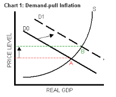
What is demand pull inflation?
occurs when demand for a good or service outstrips supply. As demand increases, sellers start selling out of the product, and frustrate potential customers. What is cost push inflation? is when a shortage of supply of labor, raw materials or capital drives up prices. The demand remains the same, but since there are fewer goods or services, the supplier can charge more per unit. |
